my_vector <- c(1, 2, 3, 4, 5, 6)2 Working with Data in R
Before we can get to the nitty-gritty of working with real data, we need to familiarize ourselves with a few more essential concepts.
2.1 Functions
Last class, we assigned a vector to a variable like this:
Where my_vector is an object and \({1,2,3,4,5,6}\) is the set of values assigned to it. When you run this code in your console (or in a script file), your new variable and its assigned values are stored in short-term memory and appear in the Environment pane of RStudio.
When we assigned a single value to another variable, however, as in:
x <- 1or,
first_name = 'Wesley'we didn’t use c(). So, what exactly is c()?
Like sum() or mean(), c() is a function. Functions play an important role in all programming languages. They are snippets of code, often hidden in the background, that allow us to accomplish specific tasks, like adding up all of the numbers in a vector, taking the mean, or creating a vector. In R, c() is a function which combines values into a vector or list.
Functions give us the ability to recall previously written code to perform the same task over again. Why re-write code every time you need to use it, after all, when you could use the same code you used last time? Instead of copying and pasting code, we can put it in a function, save it somewhere, and call it when we need it.
2.1.1 Calling a Function
When we want to use a function, or ‘call’ it as we will sometimes say, we type in the name of the function, enclose arguments in a set of parentheses, and run the command. The general form looks something like this:
function([arg1], [arg2], ...)2.1.2 Using Arguments in a Function
In some cases, you may just have one argument for a function, as when you want to use the sum() function to add the elements of a vector:
sum(my_vector)[1] 21In other cases, you may have multiple arguments:
sum(my_vector, my_vector)[1] 42Arguments can be required or optional and the number of arguments and the order in which they are input depends on the specific function you are using and what you are trying to accomplish. The sum() function, for instance, returns the sum of all values given as arguments.
Arguments can also be used to specify options for a function. Take a look at the example below:
sum(my_vector, NA, my_vector)[1] NAHere we are using the sum() function to add my_vector twice, as in the previous example, but now with a missing value (NA). Because the sum of two vectors plus a missing value is unknown, we get an unknown value (NA) as the output.
If we want the sum() function to ignore the unknown value, we have to provide it with an additional, named argument which tells it to ignore NA. We can specify this by adding , na.rm = TRUE to our function call. See what happens below:
sum(my_vector, NA, my_vector, na.rm = TRUE)[1] 42We’re back to an answer of 42. The sum() function ignored the missing value, as we specified, and added the two vectors.
All functions have named arguments and an ordering to them. If you omit the name of an argument in your function call, the function processes them according to their default ordering. It is generally a good habit to specify argument names, as in the example below where the ‘x’ argument in the sum() function takes the object you are trying to sum, but it is not entirely necessary for simple functions.
sum(x = my_vector)[1] 212.1.3 Getting Help with Functions
As you progress in R, you will learn many different functions and it can be difficult to keep track of all of the different arguments. Whenever you want to know more about what a function does or what arguments it takes, simply type ?function_name into the RStudio console and you will get some useful documentation in the Help pane located in the lower-right of your RStudio window.
?sum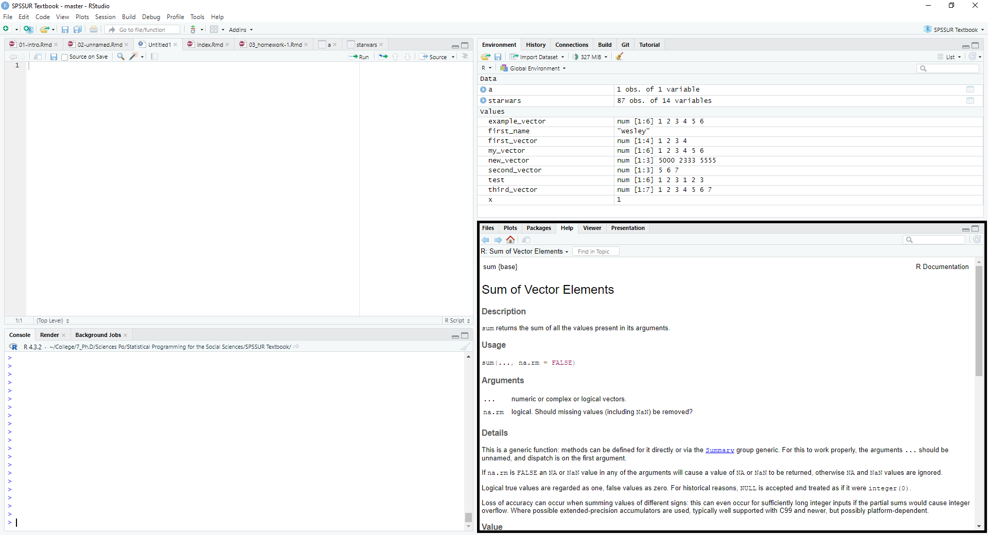
Check Your Understanding:
Let’s take a quick pause to make sure we understand what we’ve just learned.
- Create a vector of three numbers and assign it to a variable called
first_vector. Now use themean()function to find the average offirst_vector. - Now create another vector called
second_vectorwhich contains thefirst_vectorand anNAvalue. Try it on your own first, then click on this footnote to see the answer.1 - Using the
na.rm = TRUEargument, calculate the mean ofsecond_vector.
2.2 Packages
One of the great benefits of R is its power and flexibility. We’ve seen how functions provide us with the ability to reuse code, but functions are common to any programming language or statistical software.
It may sound cliché, but what makes R special is its community. R is a free and open-source software, which means that anyone can use or contribute to it. If you develop a new statistical method, for instance, you can write the code necessary to implement it and share it with others.
Base R, which you installed last class, comes with a number of built-in functions like mean(), sum(), range(), and var() . But, R users working out of the goodness of their hearts have developed many other functions that accomplish an array of tasks, from making aesthetically-pleasing visualizations to executing complex machine learning algorithms.
These functions are put together into what are called packages, which can be easily installed and loaded into R. Packages can also contain data and other compiled code.
2.2.1 Installing Packages
We’re going to use the install.packages() function to install one such package, called tidyverse.
install.packages('tidyverse')Once you’ve run this command in your RStudio console, you will have downloaded the tidyverse and saved it to your library. The library is simply where your packages are stored.
Tidyverse is actually a set of packages, including dplyr and ggplot2, all of which are useful for data analysis in R. We’ll be using the tidyverse throughout this course and you will find that it’s the most commonly used set of packages for data analysis in R.
2.2.2 Loading Libraries
Whenever you start an R session and want to use a package, you have to be sure to load it. Loading a package makes sure that your computer knows what functions and data are inside, so that you can call them at will.
To load an R package, you can use the library() function, like this:
library(tidyverse)── Attaching core tidyverse packages ──────────────────────── tidyverse 2.0.0 ──
✔ dplyr 1.1.4 ✔ readr 2.1.5
✔ forcats 1.0.0 ✔ stringr 1.5.1
✔ ggplot2 3.5.0 ✔ tibble 3.2.1
✔ lubridate 1.9.3 ✔ tidyr 1.3.1
✔ purrr 1.0.2
── Conflicts ────────────────────────────────────────── tidyverse_conflicts() ──
✖ dplyr::filter() masks stats::filter()
✖ dplyr::lag() masks stats::lag()
ℹ Use the conflicted package (<http://conflicted.r-lib.org/>) to force all conflicts to become errorsNow, that you’ve loaded tidyverse, you can access its special functions like mutate() or its data sets, like starwars. Try entering starwars in your console after you’ve loaded the tidyverse. What’s inside?
2.3 Loading Data
Great, you know what a function is, you have the tidyverse installed, and you’ve seen that data can be contained in packages, which are easy to install and load.
2.3.1 Using Data from Packages
Let’s install and load another package, so that we can take a look at some more data.
install.packages('socviz')library(socviz)The socviz package accompanies a textbook called Data Visualization written by Kieran Healy, a Professor of Sociology at Duke University, and it contains some interesting datasets including election data from the 2016 U.S. presidential election. This dataset is stored in an object titled election. Once you have socviz installed and loaded, you can get a preview of its contents by entering the name of the object:
election# A tibble: 51 × 22
state st fips total_vote vote_margin winner party pct_margin r_points
<chr> <chr> <dbl> <dbl> <dbl> <chr> <chr> <dbl> <dbl>
1 Alabama AL 1 2123372 588708 Trump Repu… 0.277 27.7
2 Alaska AK 2 318608 46933 Trump Repu… 0.147 14.7
3 Arizona AZ 4 2604657 91234 Trump Repu… 0.035 3.5
4 Arkansas AR 5 1130635 304378 Trump Repu… 0.269 26.9
5 Californ… CA 6 14237893 4269978 Clint… Demo… 0.300 -30.0
6 Colorado CO 8 2780247 136386 Clint… Demo… 0.0491 -4.91
7 Connecti… CT 9 1644920 224357 Clint… Demo… 0.136 -13.6
8 Delaware DE 10 443814 50476 Clint… Demo… 0.114 -11.4
9 District… DC 11 311268 270107 Clint… Demo… 0.868 -86.8
10 Florida FL 12 9502747 112911 Trump Repu… 0.0119 1.19
# ℹ 41 more rows
# ℹ 13 more variables: d_points <dbl>, pct_clinton <dbl>, pct_trump <dbl>,
# pct_johnson <dbl>, pct_other <dbl>, clinton_vote <dbl>, trump_vote <dbl>,
# johnson_vote <dbl>, other_vote <dbl>, ev_dem <dbl>, ev_rep <dbl>,
# ev_oth <dbl>, census <chr>For ease of use, we’re going to store a copy of this data in a new object in our environment called election_2016.
election_2016 <- electionNow, we can play around with it. In addition to getting a preview of the data by entering the name of our object in the console, we can also access it through the Environment pane of our RStudio window. Click on election_2016 and you will see the full dataset.
Just like in a spreadsheet, you can scroll through the full set of columns and rows. Remember, of course, that you cannot edit values in this view tab. This is by design. If we want to make changes to the data or perform calculations, we need to do so programmatically by using code.
2.4 Data Types and Data Structures
This seems about as good a point as any to talk about the different types of data you will encounter in R.
2.4.1 Data Types
There are six different basic data types in R. The most important for our purposes are:
- character: letters such as
'a'or sets of letters such as'apple' - numeric: numbers such as
1,1.1or23 - logical: the boolean values,
TRUEandFALSE
The other types of data are integers (which can only hold integers and take the form 1L), complex (as in complex numbers with an imaginary component, 1+2i), and raw (data in the form of bytes). You have already used the previous three and we won’t use the latter three in this course.
If you wish to check the data type, or class, of an object, you can use the class() function.
class(my_vector)[1] "numeric"2.4.2 Data Structures
There are many different data structures in R. You’ve already become familiar with one, vectors, a set of values of the same type. Other data structures include:
- list: a set of values of different types
- factor: an ordered set of values, often used to define categories in categorical variables
- data frame: a two-dimensional table consisting of rows and columns similar to a spreadsheet
- tibble: a special version of a data frame from the tidyverse, intended to keep your data nice and tidy
Note that data structures are usually subsettable, which means that you can access elements of them. Observe:
my_list <- c('a', 'b', 'c', 2)
my_list[2]
[1] "b"In the example above, we’ve called an element of the list, my_list, using an index number in a set of brackets. Since we entered the number 2 inside brackets next to our list name, we received the second element of the list, the character 'b'. We can also modify elements of a list in the same way.
Let’s now say that we want to change 'b', the second element of my_list, to the word 'blueberry':
my_list[2] <- 'blueberry'
my_list
[1] "a" "blueberry" "c" "2" Easy enough. Now try it out yourself:
- Create a vector with three elements: “sociology”, “economics”, and “psychology”
- Call each of them individually.
- Change the value of the second element to the value of the first element.
- Change the value of the third element to the value of the first element.
Be sure to do the last two programmatically rather than by re-typing the initial values.
2.5 Using Functions with Data
Back to the elections data. We have our 2016 U.S. Presidential Election data stored in a tibble called election_2016.
If we want to output a single column from the data, like state, we can do so by typing in the name of the data object (in this case, election_2016) followed by the $ symbol, and the name of the column (state).
election_2016$state [1] "Alabama" "Alaska" "Arizona"
[4] "Arkansas" "California" "Colorado"
[7] "Connecticut" "Delaware" "District of Columbia"
[10] "Florida" "Georgia" "Hawaii"
[13] "Idaho" "Illinois" "Indiana"
[16] "Iowa" "Kansas" "Kentucky"
[19] "Louisiana" "Maine" "Maryland"
[22] "Massachusetts" "Michigan" "Minnesota"
[25] "Mississippi" "Missouri" "Montana"
[28] "Nebraska" "Nevada" "New Hampshire"
[31] "New Jersey" "New Mexico" "New York"
[34] "North Carolina" "North Dakota" "Ohio"
[37] "Oklahoma" "Oregon" "Pennsylvania"
[40] "Rhode Island" "South Carolina" "South Dakota"
[43] "Tennessee" "Texas" "Utah"
[46] "Vermont" "Virginia" "Washington"
[49] "West Virginia" "Wisconsin" "Wyoming" The $ is known as a subset operator and allows us to access a single column from a table. If we want to perform a calculation on a column, we can use the column as an argument in a function like so:
# Sum the total number of votes cast in the 2016 Presidential election.
sum(election_2016$total_vote, na.rm = TRUE)
[1] 137125484Here, we summed all of the values in the total_vote column in the election_2016 tibble. The na.rm argument isn’t strictly necessary in this case (since there are no missing or unknown values), but it’s good to remember that it’s an option in case you need it.
2.6 Exercise
For the remainder of today’s session, I’d like you to play around with the election data. In particular:
- Identify the data type for the
st,pct_johnson, andwinnercolumns. - Calculate the mean
vote_marginacross the states. - Use the
table()function to count the number of states won by each presidential candidate. - Create a variable which contains the total number of votes received by Hillary Clinton (contained in the column
clinton_vote) and a variable containing the total number of votes received by Donald Trump (trump_vote). Take the difference of the two. - Create a variable containing the total number of electoral votes received by Hillary Clinton (contained in
ev_dem) and another containing the total number received by Donald Trump (ev_rep). Take the difference of the two. - Try using the
plot(x=, y=)function to plot a couple of numeric columns.
second_vector <- c(first_vector, NA)↩︎