5 Workflows and Wrangling

At this point in the course, we have primarily been working with data from packages, which is generally convenient and straight forward. We install the package with the data we want, we load the package from the library, and then we access the data and begin summarizing it. The bad news is that the data we might want to use for a particular project oftentimes isn’t contained in a package. The even worse news is that we usually need to clean and transform the data in order to get it into a format that works for analysis.

This chapter covers some of the processes and functions in R made for dealing with these unfortunate eventualities. We’ll start with the general problem of working with files in R, then learn how to get data in, and then we’ll learn more about how to make data analyzable.

This chapter will not, of course, provide you with the answers to all of the data wrangling problems you will eventually encounter. It will barely scratch the surface. But, once you manage to get data in, data wrangling becomes a matter of learning new functions and practicing the tidy data skills you’ve already started to learn.

5.1 What’s Happening Under the Hood?

Up until now, we’ve been writing our code in plain-text files saved with a .R file extension (or what we’ve been calling R script files) and we haven’t needed to load data from other files or to save anything.

That last part isn’t entirely true though. We have actually been loading data from files saved on our computers. It just so happens that the packages we installed earlier and the library() function have gone to great lengths to simplify and conceal the back-end interactions that led to data showing up in our RStudio environment. All of this data is saved somewhere on our computers, we just might not know where it is.

As with any type of computer program, R itself operates from somewhere on your hard drive. It uses data, functions, and other compiled code which have been saved across a number of files (and file types) in different locations to run the program and allow us to interact with it. This is the case for everything software-related, from the apps on your smartphone to the operating system on your laptop. It’s all running from code saved somewhere in the device’s memory.

For this chapter, we don’t have to go deep into the code that composes R or RStudio. All we need to know, instead, is how to get R to interact with files saved in different locations on our computer as well as how to organize them in a way that makes them easy to work with.

5.2 File Structures, File Paths, and the Working Directory

Your computer’s operating system (Windows, MacOS, or Linux) organizes the files on your computer into folders. You might have created some folders on your own, renamed them, or stored files like photos, documents, and other items across them. Pictures might go in a “Pictures” folder, for example, and documents in a “Documents” folder. You might have a “Sciences Po” folder and then a sub-folder for “SPSSUR.”¹

The way files are organized across folders and sub-folders on a computer’s hard drive is usually referred to as your computer’s file structure. Within a file structure, each file has a file path, which is an address that identifies where the file is located. In Windows, they usually look something like this:

"C:\Users\wcs26\Documents\Sciences Po\SPSSUR\my_file.R"

In MacOS, they might look more like this:

"/Users/wcs26/Documents/Sciences Po/SPSSUR/my_file.R"

As an important aside, when you write file paths in R, you will generally want to write them in the MacOS format you see above (i.e., using forwards slashes, /) even if you are using a PC. This is because the backwards slash, \, is a special character in R.

Within the operating systems themselves, file paths are slightly easier to find in Windows than in MacOS since you can get most of the way there by clicking in the address bar at the top of a Windows Explorer window (see below for an example).² This gives the folder path, which when followed by another slash, the file name, and the file extension, gives the file path. In MacOS, finding a file path requires a little more effort (see here for some guidance).³

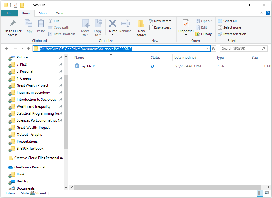
When working with multiple files in R, as you will in more involved analysis projects, you will need to pay some attention to the file structure and file paths. When you load data from a file, for instance, R will need to know exactly where the file is located. If you are saving a graph, similarly, R will need to know where you want to save it.

R makes an educated guess as to where in your file structure you are working from based on how you open your R session. This is called the working directory and you can identify where R has located it using the command below:

getwd()

Sometimes the working directory doesn’t quite match where you think it should be and you might need to change it manually as a result. We will endeavor to avoid this when we can, but if you must, you can always manually set it using setwd().

5.3 The Problem with File Paths

Functions that load data generally require you to provide a file path that leads to the data file. The problem with file structures and file paths, however, is that everyone’s is different. So, if we have a file saved in a specific location on our computer and then some code that reads it, how do we make sure that other people can use our code when their file structure is going to be different?

To make this more concrete, let’s say that I send you an R Script along with a data file called important_data.csv, so that you can replicate some analysis and visualizations I did. In that R Script, I might have a line that looks like this:

read_csv("C:/Users/wcs26/Documents/Sciences Po/SPSSUR/important_data.csv")

This command will try to read in a data file, important_data.csv, located within C:/, the Users/ folder, the wcs26/ folder, and so on and so forth. As soon as you run it, R will attempt to read the file located at the end of this path by working its way through the file structure. As soon as it hits a folder it can’t find on your computer, however, it will stop and produce an error that looks something like this:

Error: 'C:/Users/wcs26/Documents/Sciences Po/SPSSUR/important_data.csv' does not exist.

This type of file path construction, in which every folder and sub-folder on the way to the destination is provided, is called an absolute file path. If any part of the address is incorrect, R won’t be able to find the file, the file won’t be read, and the code fails to run. So, what’s the alternative?

Well, one solution is to use what are called relative file paths. A relative file path might look something like this:

read_csv("important_data.csv")

In this case, because we haven’t provided the full address, R fills in the rest by guessing and, naturally, it guesses that the missing part of the address is the working directory (i.e., C:/Users/wcs26/Documents/Sciences Po/SPSSUR/). If R guessed correctly and the file is located in your working directory, then this works perfectly fine and the data will be read correctly. If the file isn’t located in the working directory, however, it will fail.

The trouble is that sometimes you might start your R session in one place and then open files from another place. Since R can only keep track of one working directory at a time per session, it (or rather you) will get confused quickly and your relative file paths will also fail.

5.4 R Projects and `here`

Fortunately, there is a better way. To avoid these working directory problems and hard-coding absolute file paths in scripts, we’re going to use two solutions that will help keep them straight.

5.4.1 R Projects

The first is R Projects, a tool to organize your files in R Studio. When you create an R Project file (.Rproj), R Studio creates a new folder on your computer which is made to store all of the associated files you may have for a project (e.g., your data, your code, and any outputs). Every time you open that R Project file, R Studio opens a new working session with a working directory correctly set to the location of your project file. All of your files will be right where you need them.

Let’s create one for today’s classwork. In R Studio, use the navigation bar at the top of your screen to go to File > New Project > New Directory > New Project. Then, in the provided prompt, type in a project name that matches our course naming standards (e.g., “Stubenbord_Wesley_Session 5 Classwork”). Create this project as a sub-directory of your SPSSUR course folder (wherever this may be and whatever it may be called on your computer). Once this has been created, this is where your projects files will live, a permanent home just for them. You can verify that the new project folder has been created by navigating to it in your computer’s file browser (e.g., Windows Explorer in Windows).

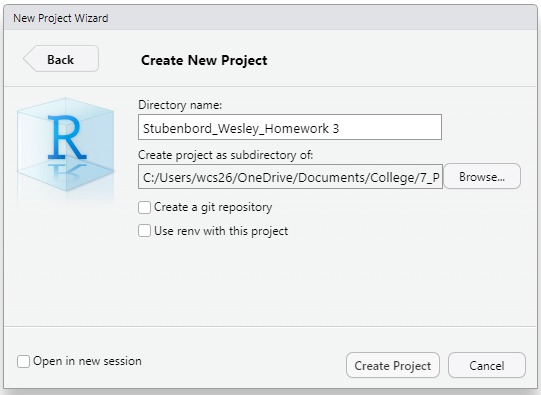
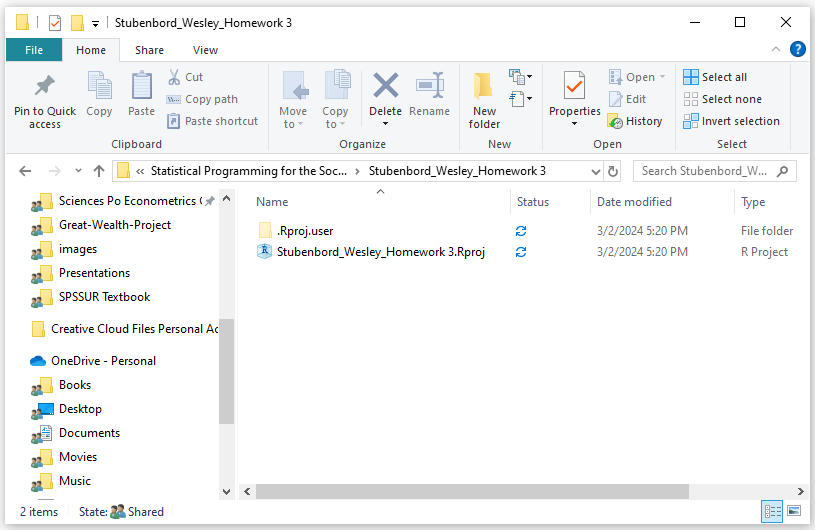
After you create a new project, you’ll find yourself in a clean R Studio session with only a console window open. The folder in your computer system will contain just the new .Rproj file and a sub-folder with some saved settings. This .Rproj file is how you will access your project from now on. Instead of opening a .R script to access your code, you’ll always want to open your .Rproj file first and then the .R script second. Don’t put anything in this new folder other than files directly associated with the project you are working on. In this case, that means that this folder is only intended to store files associated with today’s classwork.

Back in R Studio, in the lower-right hand pane with the “Files” tab, you’ll see all of the files currently associated with the project. At the moment, there shouldn’t be anything apart from the .Rproj file itself).

In this same “Files” tab, you can add a new R Script file to this project by clicking on the “New Blank File” button > “R Script”. Go ahead and create one and then save it with an appropriate file name.

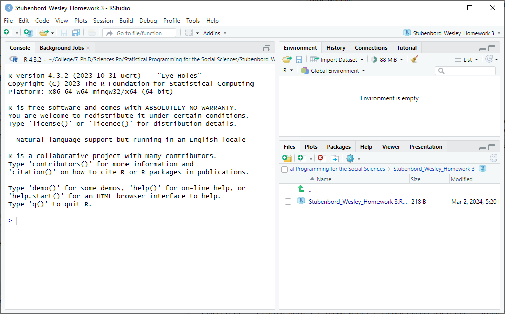
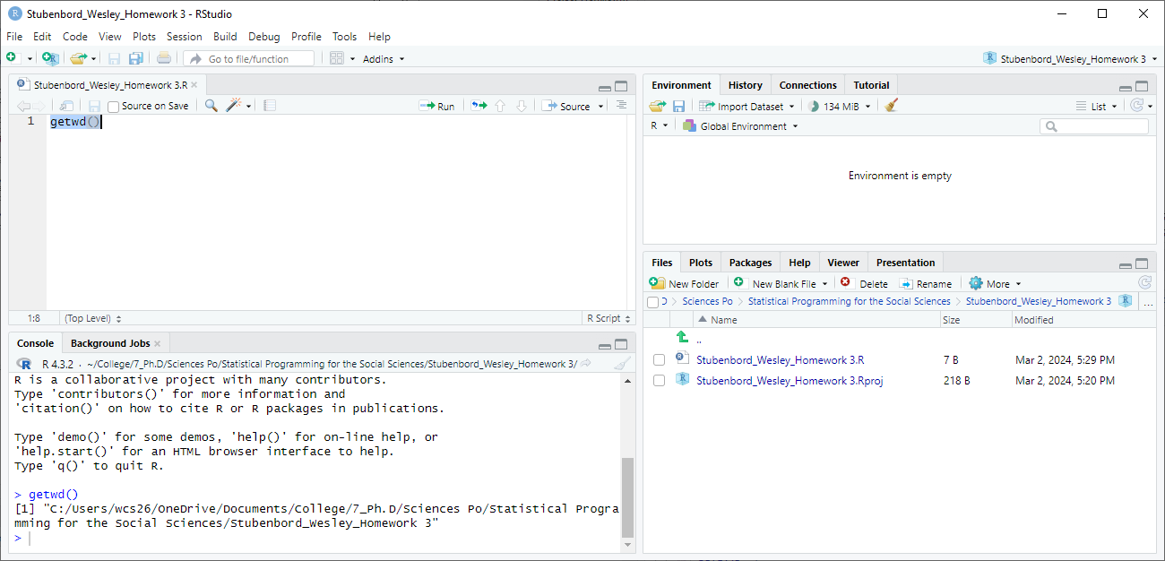
Running getwd() from your new script file or directly in the console will show you that your working directory does indeed match your R Project location. Huzzah.

5.4.2 `here`

The second tool is a package called here. here contains a useful function, called here(), which will help ensure that your code is always oriented to the correct working directory: the location of the associated R Project file. There are some occasions where, despite our best efforts, R Projects won’t save us from erroneous working directories. here helps cover those cases.

We’ll come back to the application of this function in a moment, but for now, install here, load it, and test the here() function.

#install.packages('here')
library(here)

here() starts at C:/Users/wcs26/OneDrive/Documents/College/7_Ph.D/Sciences Po/Statistical Programming for the Social Sciences/SPSSUR Textbook

here()

[1] "C:/Users/wcs26/OneDrive/Documents/College/7_Ph.D/Sciences Po/Statistical Programming for the Social Sciences/SPSSUR Textbook"

You should see, again, the correct working directory for your R Project.

5.4.3 Organizing Your Project

RProjects and here, while both extremely useful, also won’t spare you entirely from the task of organizing your project files. A clean and organized work space will make your life significantly easier in the long-run. To facilitate this, I always recommend creating a sub-folder within your project directory to store data sets (called data for example), an additional sub-folder to store figure or graphs (called figures, for example), and another to store documentation (called docs for example). These sub-folder names are commonly used among programmers and also help to ensure consistency across projects with many collaborators. You can create these folders directly in R Studio using the “New Folder” button near the top of the ‘Files’ tab in the lower-right hand pane.

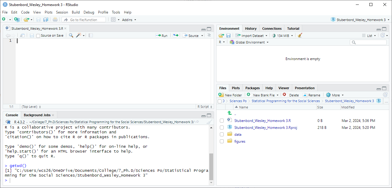
When finished, you will have your code in the main project folder along with the .Rproj file and several affiliated sub-folders for storing things later.

5.5 Getting Data into `R`

Let us get back to the primordial problem now, which is getting data into R. In the social sciences, the data we use can come from a variety of different sources: we might take our data from long-running surveys, for instance, such as the General Social Survey, the European Social Survey, or the World Values Survey. We can also use administrative data produced by government agencies, like the Federal Bureau of Investigation’s Uniform Crime Reports or data from New York City’s Open Data initiative.

Alternatively, we can use data from other sources, which may not have been produced with research or administrative purposes in mind. For example, we can scrape data from social media to see how political sentiment changes in times of crises or we can use data from online dating apps to see how social norms around courtship have changed.

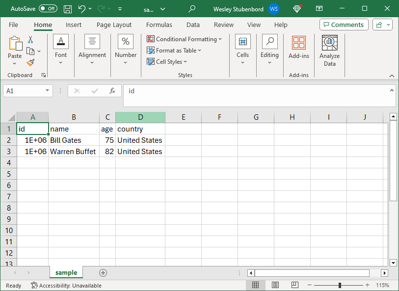
In any case, the most common format you are likely to find data stored in is a CSV file, which stands for comma separated values. CSVs are particularly appealing for data storage because they are lightweight and they are simple. They don’t contain any extra formatting - all they consist of is plain-text data in rows (separated by new lines) and columns (separated by commas). A CSV file could consist of the following, for example:

"id","name","age","country"
1011232,"Bill Gates",75,"United States"
1022234,"Warren Buffet",82,"United States"

When you open a CSV file in software like Microsoft Excel, it is usually automatically parsed into different columns, based on the position of the commas, and into different rows, based on the line breaks.⁴ Excel will automatically recognize, for example, that name is a column containing two values, “Bill Gates” in one row and “Warren Buffett” in another. CSVs don’t always use commas to separate their values - sometimes (especially in Europe), they use semi-colons. The character (e.g., , or ;) that separates values in a data file is called a delimiter.

5.6 Loading files from CSVs

Thankfully, loading CSV files is not very difficult in R. R has a base function for loading CSVs, read.csv(), but there is a better version called read_csv() which comes from the readr package. readr is also located in the tidyverse, but must also be loaded separately, just like the scales package in the previous chapter.⁵

On the course Moodle site, you’ll find a CSV titled billionaires_2020-2023.csv, which contains some limited data on the world’s billionaires from my own research. Go ahead and download this file and then save it in the data sub-folder you created in your Session 5 Classwork project folder. Open the Session 5 Classwork project and a script file inside of it, if you haven’t already. We’ll load a few libraries first and then the data set.

library(tidyverse)

── Attaching core tidyverse packages ──────────────────────── tidyverse 2.0.0 ──
✔ dplyr     1.1.4     ✔ readr     2.1.5
✔ forcats   1.0.0     ✔ stringr   1.5.1
✔ ggplot2   3.5.0     ✔ tibble    3.2.1
✔ lubridate 1.9.3     ✔ tidyr     1.3.1
✔ purrr     1.0.2     
── Conflicts ────────────────────────────────────────── tidyverse_conflicts() ──
✖ dplyr::filter() masks stats::filter()
✖ dplyr::lag()    masks stats::lag()
ℹ Use the conflicted package (<http://conflicted.r-lib.org/>) to force all conflicts to become errors

library(readr)
library(here)

As with any function that reads data, read_csv() requires a file path to locate the data and read it into our R session. Because the data set is located in a sub-folder and because we want to use a relative path (rather than an absolute path), we’ll use here().

Remember, here() provides the file path to your R Project folder. Any additional folder or file names used as arguments inside of the here() function (separated by a comma) will be added to the project folder path. If your R Project folder is located at C:\Users\Documents\My Projects, for example, here("data") will output C:\Users\Documents\My Projects\data. You must enclose the name of your sub-folders in quotation marks.

Entering the following should return the file path of the data set if you have saved it within your data subfolder:

here("data","billionaires_2020-2023.csv")

[1] "C:/Users/wcs26/OneDrive/Documents/College/7_Ph.D/Sciences Po/Statistical Programming for the Social Sciences/SPSSUR Textbook/data/billionaires_2020-2023.csv"

To read the actual data into R, now all we need to do is put this here function inside of read_csv() in the file = argument.

read_csv(file = here("data","billionaires_2020-2023.csv"))

Rows: 2640 Columns: 13
── Column specification ────────────────────────────────────────────────────────
Delimiter: ","
chr (8): name, gender, country, countrycode, region, marital, residence_coun...
dbl (5): id, 2020, 2021, 2022, 2023

ℹ Use `spec()` to retrieve the full column specification for this data.
ℹ Specify the column types or set `show_col_types = FALSE` to quiet this message.

# A tibble: 2,640 × 13
      id name        gender country countrycode region marital residence_country
   <dbl> <chr>       <chr>  <chr>   <chr>       <chr>  <chr>   <chr>            
 1     1 A. Jayson … male   United… USA         North… Married United States    
 2     9 Abdulla Al… male   United… ARE         Middl… Married United Arab Emir…
 3    10 Abdulla bi… male   United… ARE         Middl… <NA>    United Arab Emir…
 4    12 Abdulsamad… male   Nigeria NGA         Sub-S… Married Nigeria          
 5    13 Abhay Firo… male   India   IND         South… Married India            
 6    14 Abhay Soi   male   India   IND         South… <NA>    <NA>             
 7    16 Abigail Be… female United… USA         North… <NA>    <NA>             
 8    17 Abigail Jo… female United… USA         North… Married United States    
 9    18 Abilio dos… male   Brazil  BRA         Latin… Married Brazil           
10    20 Acharya Ba… male   India   IND         South… Single  India            
# ℹ 2,630 more rows
# ℹ 5 more variables: selfmade <chr>, `2020` <dbl>, `2021` <dbl>, `2022` <dbl>,
#   `2023` <dbl>

As you can see from the output above, read_csv() worked! If our data had used a semi-colon as a delimiter instead of a comma, we would have just used read_csv2() instead.

We can see from the resulting output that this data set has 2,640 rows and 13 columns. Let’s save this into a new object in our environment.

billionaires <- read_csv(file = here("data","billionaires_2020-2023.csv"))

Rows: 2640 Columns: 13
── Column specification ────────────────────────────────────────────────────────
Delimiter: ","
chr (8): name, gender, country, countrycode, region, marital, residence_coun...
dbl (5): id, 2020, 2021, 2022, 2023

ℹ Use `spec()` to retrieve the full column specification for this data.
ℹ Specify the column types or set `show_col_types = FALSE` to quiet this message.

You’ll notice that read_csv() says a lot each time you run it. Don’t confuse the red text you see here with errors, however. It’s just trying to be helpful by giving you some more information about the data we’re reading in. We can see from this output, for example, that there are 8 character columns and 5 dbl columns. dbl stands for double and is a type of numeric value. We can, of course, use glimpse() to see the variables again along with some of the first few values.

glimpse(billionaires)

Rows: 2,640
Columns: 13
$ id                <dbl> 1, 9, 10, 12, 13, 14, 16, 17, 18, 20, 25, 26, 27, 29…
$ name              <chr> "A. Jayson Adair", "Abdulla Al Futtaim", "Abdulla bi…
$ gender            <chr> "male", "male", "male", "male", "male", "male", "fem…
$ country           <chr> "United States", "United Arab Emirates", "United Ara…
$ countrycode       <chr> "USA", "ARE", "ARE", "NGA", "IND", "IND", "USA", "US…
$ region            <chr> "North America", "Middle East & North Africa", "Midd…
$ marital           <chr> "Married", "Married", NA, "Married", "Married", NA, …
$ residence_country <chr> "United States", "United Arab Emirates", "United Ara…
$ selfmade          <chr> "self-made", "self-made", "inherited", "self-made", …
$ `2020`            <dbl> NA, 2.437, 4.293, 3.365, 1.740, NA, NA, 12.531, 2.66…
$ `2021`            <dbl> 1.110, 2.441, 3.107, 5.437, 2.663, NA, NA, 23.189, 2…
$ `2022`            <dbl> 1.140, 2.591, 2.695, 7.151, 2.902, NA, NA, 21.971, 2…
$ `2023`            <dbl> 1.3, 2.4, 3.0, 8.2, 2.7, 1.2, 1.1, 21.6, 2.4, 3.4, 2…

There are other ways you can take a peek at your data. We can take a random slice of the data using slice_sample() from dplyr, for example. We can also use slice_head() to see the first few rows, slice_tail() to see the last few rows, or slice_min() and slice_max() to see the rows with the largest or smallest values for some variable. Give them each a try and look at their documentation to see some helpful optional arguments you can use as well, like n =.

billionaires %>%
  slice_sample(n = 5)

# A tibble: 5 × 13
     id name         gender country countrycode region marital residence_country
  <dbl> <chr>        <chr>  <chr>   <chr>       <chr>  <chr>   <chr>            
1   184 Ana Lucia d… female Brazil  BRA         Latin… Married Brazil           
2  2076 John Ruiz    <NA>   United… USA         North… <NA>    <NA>             
3  1733 Igor Makarov male   Russia  RUS         Europ… Married United States    
4  2979 Michael Mor… male   United… USA         North… Married United States    
5  3654 Roman Trots… male   Russia  RUS         Europ… Married Russia           
# ℹ 5 more variables: selfmade <chr>, `2020` <dbl>, `2021` <dbl>, `2022` <dbl>,
#   `2023` <dbl>

No matter how we choose to do it, though, our purpose at this point of reading data in should always be to get a sense for any potential issues lurking beneath the surface of our data file.

You may have noticed from glimpse that there is something a little bit weird about this data. Four columns at the end have numbers as titles. What are these columns? Since this data doesn’t come from a package and there’s no documentation, I will tell you: they’re the estimated net worth of each of the listed individuals in billions of 2023-inflation adjusted dollars for each of the named years (i.e., 2020, 2021, 2022, 2023). The values are in billions of US dollars.⁶

Now that we know what the data is, we can start to make sense of it. We can use slice_max() , for instance, to see who was the richest person in 2023. In this case, note that when we reference a variable which begins with a number, we have to use the ` character to enclose the variable name. This is because R does not allow object names to start with a number.

billionaires %>%
  slice_max(`2023`, n = 1)

# A tibble: 1 × 13
     id name         gender country countrycode region marital residence_country
  <dbl> <chr>        <chr>  <chr>   <chr>       <chr>  <chr>   <chr>            
1   425 Bernard Arn… male   France  FRA         Europ… Married France           
# ℹ 5 more variables: selfmade <chr>, `2020` <dbl>, `2021` <dbl>, `2022` <dbl>,
#   `2023` <dbl>

Now we can see that Bernard Arnault was the richest person in 2023 with an estimated net worth of $211 billion. What if we want to see what the cumulative net worth of all French billionaires was for the years covered in this data? Maybe we could use dplyr to summarize:

billionaires %>%
  group_by(country) %>%
  filter(country == "France") %>%
  summarize(total_nw = sum())

# A tibble: 1 × 2
  country total_nw
  <chr>      <int>
1 France         0

Here we run into a problem. We can’t group_by(country, year), because there is no variable called year. There’s also no net_worth variable that we can put into our summarize() function. So, we’re stuck with bad options. We could try something like this, for example:

billionaires %>%
  group_by(country) %>%
  filter(country == "France") %>%
  summarize(nw_2023 = sum(`2023`),
            nw_2022 = sum(`2022`),
            nw_2021 = sum(`2021`),
            nw_2020 = sum(`2020`))

# A tibble: 1 × 5
  country nw_2023 nw_2022 nw_2021 nw_2020
  <chr>     <dbl>   <dbl>   <dbl>   <dbl>
1 France     585.      NA      NA      NA

That got us the total net worth of French billionaires in 2023, at least, but it didn’t calculate a result for the other years. The reason why we’re having a hard time here is that our data is not in the right format for tidyverse functions.

5.7 Tidy Data

In the previous chapter, we learned that the gapminder data was in just the right format for ggplot. We called this long format data, which is usually how we describe this format in the social sciences. In a long format, rows are repeated observations for some unit of analysis (like a country) across some dimension (like time). In the case of the gapminder data, each of these observations (country-years) had a value for a set of variables of interest (e.g., life expectancy and GDP per capita) as shown below.

country	year	lifeExp	gdpPercap
France	1952	67.41	7029.809
France	1957	68.93	8662.835
France	1962	70.51	10560.486
France	1967	71.55	12999.918
France	1972	72.38	16107.192

In the billionaires data, we instead have one row per unit of analysis (billionaires) and multiple columns for a single variable of interest (net worth).

id	name	2020	2021	2022	2023
1	A. Jayson Adair	NA	1.110	1.140	1.3
9	Abdulla Al Futtaim	2.437	2.441	2.591	2.4
10	Abdulla bin Ahmad Al Ghurair	4.293	3.107	2.695	3.0

The column titles (e.g., 2020, 2021), to be clear, are not actually different variables, they are simply values of a single variable (e.g., year). When data is split in this way, we say it is in a wide format. Wide data does have its uses. It is very convenient, for instance, for storing a large amount of data in a small amount of space - a particular concern when you are printing data sets. Long data, on the other hand, is much better for data analysis.

The tidyverse functions require data to be in what Hadley Wickham and collaborators call a tidy format. In tidy data, each variable is in a column, each observation is in a row, and each cell contains a single value (Wickham et al. 2019). It is, in other words, in a consistent long-format. If we want to be able to use all of the great features of dplyr and ggplot, we need to transform our data into a tidy format.

5.8 Pivoting from Wide to Long

Fortunately, dplyr has some handy functions for this. Since we have data in a wide format and wish to change it to a long format, we’ll need to use a function called pivot_longer(). There are three arguments we need to provide to pivot_longer().

First, in the cols = argument, we need to provide the columns we are trying to combine into a single variable. In our case, our net worth values are distributed across the `2020`, `2021`, `2022`, and `2023` columns, so we’ll put those in a vector and use them for this argument. Next, in the names_to = argument, we need to identify where we want to put the names for each of those values (in other words, the titles for each of our former columns). Since each of those column names corresponds to a year, we’ll tell it to put them in a "year" column. Last, we need to specify a name for the variable holding all of the values that were stored across those columns. Since the values were net worth, we’ll call this new variable net_worth. We might also want to drop the rows which contain NA values for net worth and so we’ll add an optional fourth argument, values_drop_na =.

billionaires %>%
  pivot_longer(cols = c(`2020`, `2021`, `2022`, `2023`),
               names_to = "year",
               values_to = "net_worth",
               values_drop_na = TRUE)

# A tibble: 9,142 × 11
      id name        gender country countrycode region marital residence_country
   <dbl> <chr>       <chr>  <chr>   <chr>       <chr>  <chr>   <chr>            
 1     1 A. Jayson … male   United… USA         North… Married United States    
 2     1 A. Jayson … male   United… USA         North… Married United States    
 3     1 A. Jayson … male   United… USA         North… Married United States    
 4     9 Abdulla Al… male   United… ARE         Middl… Married United Arab Emir…
 5     9 Abdulla Al… male   United… ARE         Middl… Married United Arab Emir…
 6     9 Abdulla Al… male   United… ARE         Middl… Married United Arab Emir…
 7     9 Abdulla Al… male   United… ARE         Middl… Married United Arab Emir…
 8    10 Abdulla bi… male   United… ARE         Middl… <NA>    United Arab Emir…
 9    10 Abdulla bi… male   United… ARE         Middl… <NA>    United Arab Emir…
10    10 Abdulla bi… male   United… ARE         Middl… <NA>    United Arab Emir…
# ℹ 9,132 more rows
# ℹ 3 more variables: selfmade <chr>, year <chr>, net_worth <dbl>

If we take a look at the data now, we can see that we’ve increased our number of rows substantially (to 9,142) and each net worth value is now in a separate row according to the corresponding year and individual. It looks tidy. Now we can do much of the same type of data analysis and visualization we have been doing over the past couple of chapters.

# A quick and dirty plot.
tidy_bil <- billionaires %>%
  pivot_longer(cols = c(`2020`, `2021`, `2022`, `2023`),
               names_to = "year",
               values_to = "net_worth",
               values_drop_na = TRUE)

tidy_bil %>%
  group_by(country, year) %>%
  filter(country == "France") %>%
  summarize(agg_nw = sum(net_worth)) %>%
  ggplot(mapping = aes(x = year, y = agg_nw, group = country)) + 
  geom_line(linewidth = 2) +
  labs(title = "The Wealth of France's Billionaires",
       x = "Year",
       y = "Net Worth (USD in Billions)") + 
  theme_minimal()

`summarise()` has grouped output by 'country'. You can override using the
`.groups` argument.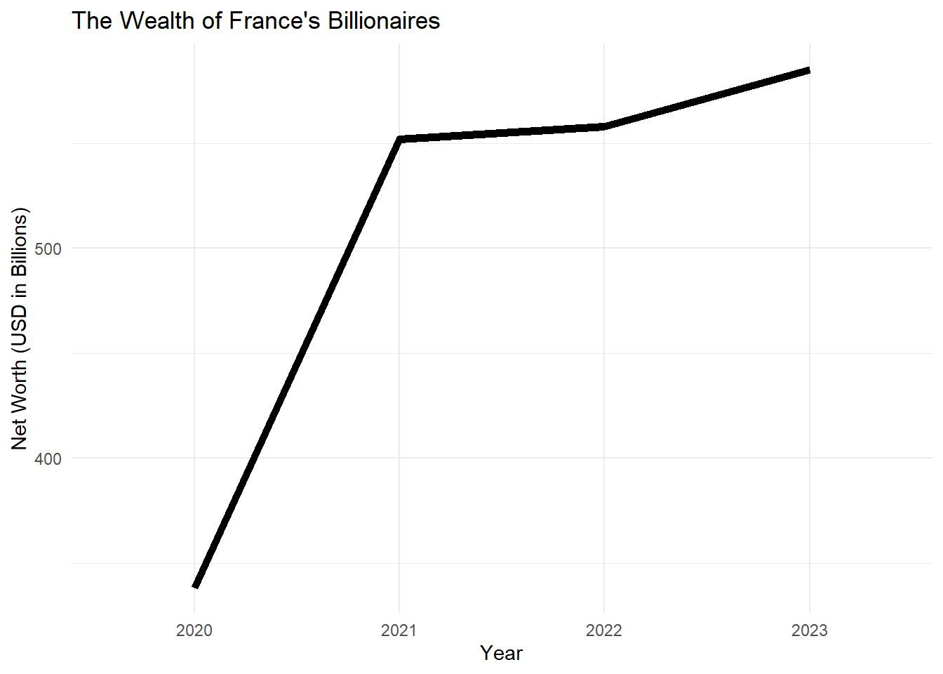

5.9 Merging Data

Let’s say that we want to do some further analysis involving additional data not contained in the data set we are currently using. Can we add it to our existing data set? The answer is yes.

On the course Moodle site, you’ll find another data set called age.xlsx. This is an Excel file. Fortunately, the readxl package (also contained in the tidverse and requiring separate loading) has just the function. Download the file from the Moodle page, add it to your project’s data folder, and then use the command below:

library(readxl)

Warning: package 'readxl' was built under R version 4.3.3

bil_age <- read_xlsx(path = here("data", "age.xlsx"), sheet = "Sheet1")

glimpse(bil_age)

Rows: 2,724
Columns: 3
$ id   <dbl> 1, 9, 12, 13, 14, 16, 17, 18, 20, 25, 26, 27, 29, 32, 33, 34, 36,…
$ year <dbl> 2023, 2023, 2023, 2023, 2023, 2023, 2023, 2023, 2023, 2023, 2023,…
$ age  <dbl> 53, 83, 62, 78, 49, 42, 61, 86, 50, 40, 44, 81, 39, 54, 52, 39, 6…

As we can see from the output, there isn’t too much in here, just an ID, a year, and an age. If we want to use this data in our next analysis, we now need to merge it with our previously tidied data. We might just want to check the year column to see how many years this age data covers.

bil_age %>%
  distinct(year)

# A tibble: 2 × 1
   year
  <dbl>
1  2023
2    NA

#An alternative way:
#unique(bil_age$year)

There’s only one year, unfortunately, and quite a few missing values. Before we go ahead and merge, we should also check to make sure that there is only one age value for each ID. Merging data with multiple values for each unit of analysis will cause rather large problems. Keep a careful eye on your data as you do these types of things. The code below will count the number of rows:

bil_age %>%
  count(id) %>%
  filter(n > 1)

# A tibble: 59 × 2
      id     n
   <dbl> <int>
 1     1     4
 2     9     2
 3    12     5
 4    13     5
 5    14     2
 6    15     2
 7    16     2
 8    17     5
 9    18     5
10    19     2
# ℹ 49 more rows

It looks like there are a few duplicates in here. We can investigate further, but let’s see if dropping the NAs fixes our problem. They won’t be useful in our analysis later anyways.

bil_age %>%
  drop_na(age) %>%
  count(id) %>%
  filter(n > 1)

# A tibble: 0 × 2
# ℹ 2 variables: id <dbl>, n <int>

Good, no results, which means that dropping the NAs solved our problem with duplicates. Let’s save the tibble without the missing values and carry on with our merge.

bil_age %>%
  drop_na(age) -> bil_age

Note that we’ve used our assignment operator in a somewhat unorthodox way here. Instead of using it at the beginning of the piped function, we’ve added it to the end. This works and is also acceptable.

Now, let’s merge. Here, we’ll use a function from dplyr called left_join(). There are other types of _join() functions depending on the use case. In our case, we have an existing data set and we simply want to add data from another tibble to it. We don’t care much about what happens to the rows in the bil_age data set that don’t match up. We’ll use left_join() as a result. Other types of joins include right_join(), inner_join(), left_join() and full_join(). Take a look at the supporting documentation to learn more about them.

left_join(x = tidy_bil, 
          y = bil_age, 
          join_by(id, year))

This didn’t quite work and, if we look at our error, we can see why. The year column in our tidy_bil data is a character and the the year column in our age data is a double. We’ll have to convert the column in tidy_bil to continue. We should probably convert year to a date format, but we’re going to cheat here and just convert it to a numeric variable for convenience. Hopefully this won’t come back to bite us later.

tidy_bil %>%
  mutate(year = as.numeric(year)) -> tidy_bil

Let’s try the merge again:

tidy_bil <- left_join(x = tidy_bil, 
                      y = bil_age, 
                      join_by(id, year))
# An alternative way to do this is:
#tidy_bil <- tidy_bil %>%
#  left_join(bil_age,
#            join_by(id, year))

Success! Whenever you do these sorts of things, try running the code without re-assigning it back to the original object first and then assign it once you are sure it works. Otherwise, you may start running into unexpected errors as you change your data. You can always re-load it if you’ve made a mistake somewhere.

If we take a look at tidy_bil, we can now see that we have an age column. Now we can do something like this:

p <- ggplot(data = tidy_bil,
            mapping = aes(x = age,
                          y = net_worth))

p + geom_point() + theme_bw()

Warning: Removed 6569 rows containing missing values or values outside the scale range
(`geom_point()`).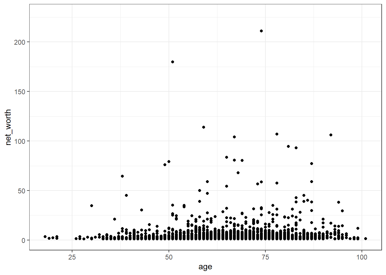

# An alternative way to do this is:
#tidy_bil %>%
#  ggplot(mapping = aes(x = age,
#                       y = net_worth)) +
#  geom_point() + theme_bw()

Notice that here we are also using ggplot() in a different way from the previous chapter. In this case, we first save our base ggplot() layer to an object (arbitrarily named p) and then we add layers to the object in a separate line of code. You’ll see this method used often in references elsewhere. Either style of writing your ggplot() code is fine, but I tend to prefer the piped form, since it allows you to add filters and do other data manipulations in the same piped command generating the plot. This is a stylistic and workflow preference though. You will find many such forking paths as you continue to learn R.

A more general understanding to take away from this example, however, is the fact that since we aren’t using a piped function, we do need to specify a data = argument in the ggplot() function. The use of the pipe operator ordinarily absolves us of having to specify a data argument in all dplyr functions, since the pipe operator does it for us (i.e., “take this AND THEN...”).

To use a filter on a tibble, for example, you could simply enter filter(data = tidy_bil, year == 2020) as a stand-alone command and it would give you the same answer as tidy_bil %>% filter(year == 2020). The pipe operator simply makes for more efficient data analysis by allowing us to string together several of these types of functions.

5.10 Pivoting from Long to Wide

Let’s say we want to compare the net worth of billionaires in our data set by marital status. We could use our data in wide format for this (billionaires). Let’s imagine that we don’t have the wide data though. Could we transform our long data into a wide format? Yes, using pivot_wider():

tidy_bil %>%
  pivot_wider(
    names_from = year,
    values_from = net_worth
  )

# A tibble: 5,040 × 14
      id name        gender country countrycode region marital residence_country
   <dbl> <chr>       <chr>  <chr>   <chr>       <chr>  <chr>   <chr>            
 1     1 A. Jayson … male   United… USA         North… Married United States    
 2     1 A. Jayson … male   United… USA         North… Married United States    
 3     9 Abdulla Al… male   United… ARE         Middl… Married United Arab Emir…
 4     9 Abdulla Al… male   United… ARE         Middl… Married United Arab Emir…
 5    10 Abdulla bi… male   United… ARE         Middl… <NA>    United Arab Emir…
 6    12 Abdulsamad… male   Nigeria NGA         Sub-S… Married Nigeria          
 7    12 Abdulsamad… male   Nigeria NGA         Sub-S… Married Nigeria          
 8    13 Abhay Firo… male   India   IND         South… Married India            
 9    13 Abhay Firo… male   India   IND         South… Married India            
10    14 Abhay Soi   male   India   IND         South… <NA>    <NA>             
# ℹ 5,030 more rows
# ℹ 6 more variables: selfmade <chr>, age <dbl>, `2021` <dbl>, `2022` <dbl>,
#   `2023` <dbl>, `2020` <dbl>

We’ll just use the original data anyways though. To see what values are in our marital variable, we can use this:

billionaires %>%
  distinct(marital)

# A tibble: 9 × 1
  marital           
  <chr>             
1 Married           
2 <NA>              
3 Single            
4 Widowed           
5 Separated         
6 Divorced          
7 Widowed, Remarried
8 In Relationship   
9 Engaged

There are 9 distinct categories. Nine is perhaps too many. What if we decide we want to use just three categories: “Married/Widowed”, “Single”, and “Other” instead?

5.11 `Recoding Using case_match()`

Recoding is useful when the categories within a data set aren’t quite appropriate for how we want to analyze them. To recode our data according to our new groupings, we can use the case_match() function inside of a dplyr mutate() function. Essentially, we are modifying a column so that the values of the new column take on the recoded values of the old column. We could mutate the original column directly (in this case, marital), but it’s generally best practice to put our recoded values inside of their own new column to make sure we don’t make a mistake. Otherwise, we’d have to reload our data and re-run all of the other code in our analysis up to this point. That can get annoying quickly. We’ll call the recoded variable marital_rc.

The first argument in case_match() is the column that needs to be recoded. The following arguments, which contain the recoding scheme, follow the format old_values ~ new_values. The original values go on the left-hand side and the values to be recoded go on the right. To separate the left and right-hand sides, we use a ~ character and a comma to separate each set of old and new values. Since we are re-coding multiple old values at a time, we’ll also put those sets of old values inside of vectors. Remember, test this without re-assigning the result to your original object first and then re-assign it once you are confident you’ve done it correctly.

billionaires %>%
  mutate(
    marital_rc = case_match(marital,
                            c('Married', 'Widowed, Remarried', 'Widowed') ~ 'Married/Widowed',
                            c('Single') ~ 'Single',
                            c('Engaged', 'In Relationship', 'Divorced', 'Separated') ~ 'Other')) -> billionaires

Did it work correctly?

billionaires %>%
  distinct(marital_rc)

# A tibble: 4 × 1
  marital_rc     
  <chr>          
1 Married/Widowed
2 <NA>           
3 Single         
4 Other

Yes, we’ve recoded successfully. There seem to be some missing values in our data, but we don’t necessarily want to drop them. Let’s make a quick graph showing median net worth with our recoded marital status variable for 2023.

billionaires %>%
  group_by(marital_rc) %>%
  summarize(median_nw = median(`2023`)) %>%
  ggplot(mapping = aes(x = marital_rc,
                       y = median_nw,
                       fill = marital_rc)) +
  geom_col() + theme_minimal()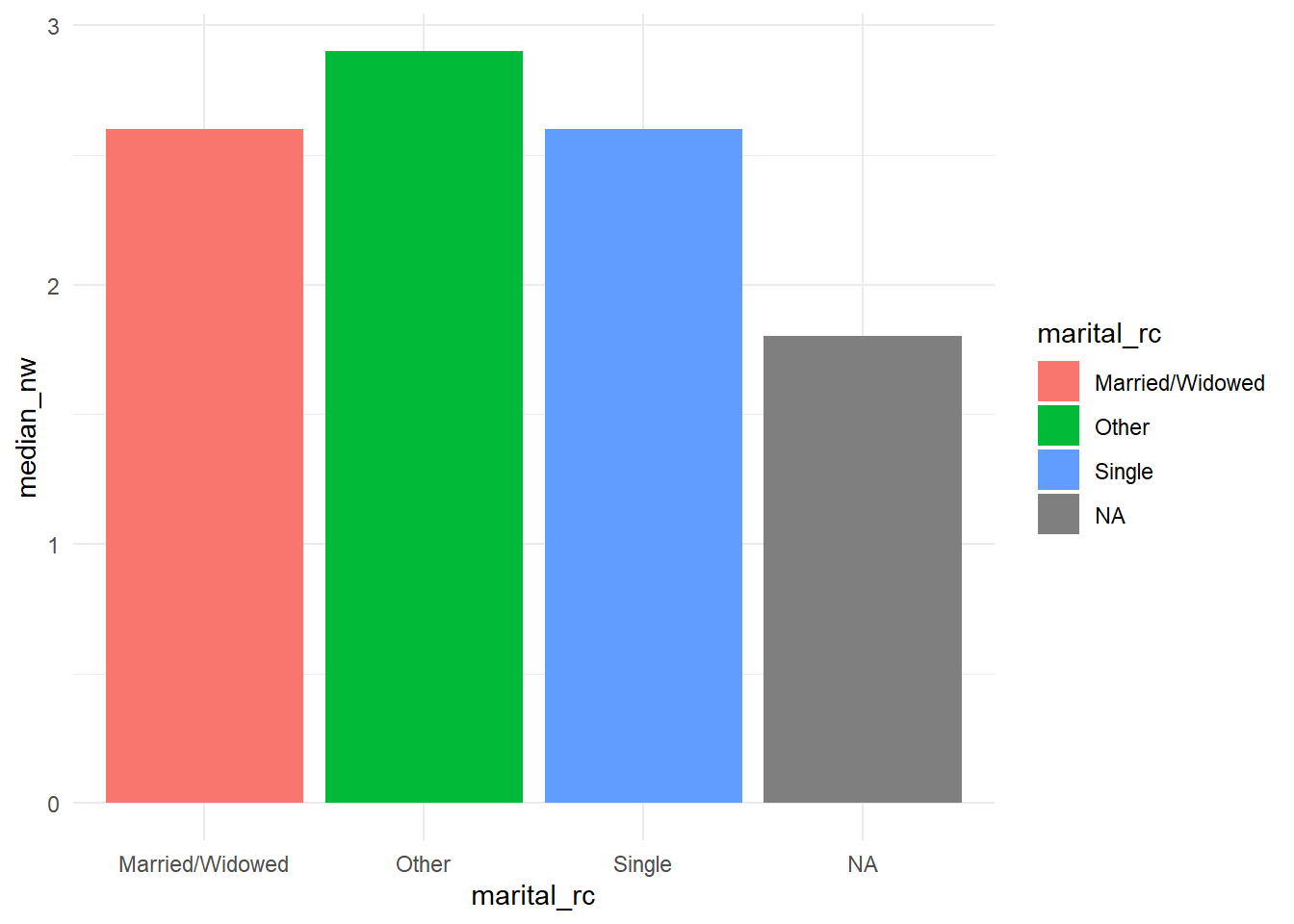

Note, of course, that we can’t make any claims about associations here. There are a lot of missing values (NA) and we don’t know whether they would be biased towards a particular category. Our Other category is also quite expansive and perhaps not analytically appropriate.

Last, but not least, we don’t know whether any of the visual differences we are seeing in median net worth across category are due to random chance alone or due to some relationship between the variables. We’ll return to this latter point in the next chapter when we start talking about inferential methods.

5.12 Exercises

For the remainder of class or for homework, keep playing around with this data to practice the new functions you’ve learned and the dplyr functions you’ve learned in previous chapters.

You may also have all of your files saved on your “Desktop” folder, in which case, you should consider applying the Marie Kondo principles of tidying up to your digital spaces. A minor caveat, though, which is that sparking joy may not be a good criteria for computer system files.↩︎
Note that if you copy and paste a path from a Windows Explorer into R, you’ll have to change the direction of the \ to / or deal with the \ issue in a different way (there are other ways, but hopefully you won’t need to copy and paste paths anyways).↩︎
If you are using a Linux-based OS, you probably won’t need an explanation of file structures and file paths, given the greater transparency of file paths and structures you regularly encounter.↩︎
Parsing refers to how software reads the values.↩︎
As before, rather than load the entire readr package via library(), you can also use the :: syntax, as in readr::read_csv().↩︎
The net worth estimates here are derived from the Forbes’ annual World’s Billionaires list and inflation-adjusted using an implict GDP price deflator from the U.S. Federal Reserve.↩︎